pp2web
What is it?
pp2web (post-processing to web) is a server-side web app for post-processing data from raw sessions, such as those acquired with the mobile app rawX, in the following modes:
- Single
- Static
- Kinematic
- Stop&Go (new)
How is it used?
After registering by e-mail at solutop@gmail.com you can ask for a trial (time-limited) or perpetual activation. Once you have your credentials, use the following link to log in.
pp2web lets you:
- choose the post-processing mode (Single, Static, Kinematic, Stop&Go)
- upload a raw rover file in .ubx format (Single, Static, Kinematic)
- upload a master RINEX file in .YYo or .obs format (Static, Kinematic and Stop&Go only)
- upload a file with the Stop and Go intervals of the rover in .csv format (Stop&Go only)
- enter LLE if you know the precise geographic coordinates of the master station (Static, Kinematic and Stop&Go only)
- process the uploaded file or files
- display the points on OSM on screen
- download a zip file holding both the .csv file and a PDF report typeset in LaTeX
- restart the app to use it again
Relative positioning
Let us take a small step back and see what relative positioning is.
GNSS post-processing refers to relative positioning techniques, which determine the difference in coordinates (the baseline) between two or more points occupied at the same time by several receivers able to acquire both code and phase.
It can be done either statically (the receivers are kept in position for a measurement session lasting from a few minutes to several hours depending on the length of the baseline) or kinematically (one receiver stays fixed while the other, or the others, move, occupying the points to be surveyed one after another or following a continuous path).
Note
The computation is carried out in post-processing (after the event, so not in real time) starting from the raw data acquired by the receivers. Static mode can reach a relative positioning accuracy of the order of 0.5-1 cm and is used to determine networks of baselines for framing purposes or for deformation monitoring.
Kinematic mode is used above all to reconstruct routes and the kinematics of vehicles (road cadastre, study of vehicle motion and so on). Below is an example of relative positioning
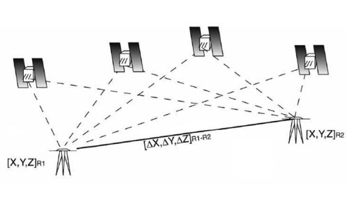
Fig.1 The GNSS relative positioning technique
In the figure above the two receivers observe the same satellites at the same instant. Those observations are then processed to estimate the baseline (a 3D vector) between the two receivers.
Hint
The way the rover measures determines the positioning technique. GNSS is often used as a black box: the measurement is recorded without knowing its limits, so it is worth spending some time understanding how this positioning technique works.
The accuracy depends on:
- the type of receivers (which observables they can acquire)
- the distance between the receivers (from < 10 km to > 500 km)
- the survey method (how long each point is occupied)
- the data processing approach (real time, post-processing)
- 1-2 m (relative, on the codes, in real time), used in navigation
- a few centimetres (dual frequency, rapid static), surveying and GIS work
- millimetric (dual frequency, long static sessions with adjustment techniques), crustal deformation
Reminder
- post-processing applies to surveys acquired in relative positioning
- for every point of the survey the phase recordings (also called observables or observations) are required, and the code ones are recommended too.
- information about the orbits of the navigation satellites is required (brdc files, holding the orbit parameters, and sp3 files, holding the orbit trajectories)
- the recordings have to be taken at the same time on one or more points of known coordinates and on the points being surveyed
- the integer phase ambiguity is resolved by the processing software
- the occupation time is essential in order to resolve the integer phase ambiguity
- the occupation times depend on the type of receiver, on the length of the baseline, on the satellite geometry and on any sources of multipath
Stop&Go
Stop&Go is a surveying technique using two geodetic GNSS receivers (one fixed and one moving) that exploits carrier phase observations to obtain very precise coordinates.
Note
Unlike static mode, in which the rover stays still for 10-30 minutes on each point, in Stop&Go the rover stops briefly (10-30 seconds) on each point after an initial ambiguity fixing stage.
Operating stages
- a. Initialisation (fixing the ambiguities)
- You start from a known or control point.
- The rover stays still for 2 to 5 minutes so that the software can resolve the integer ambiguities (the whole number of carrier cycles between satellites and receivers).
- Once the fix is achieved (a “fixed” solution), you can go on to survey the following points.
- b. Moving between points (Go)
- The operator walks to the new point without switching the receiver off or interrupting it, keeping the observations continuous.
Warning
- It is essential never to lose the signal or the fixed solution. Going through tunnels or under dense trees, or otherwise blocking the view of the satellites, can lose the fix.
- c. Surveying the points (Stop)
- On each point of interest the rover is set up and held steady for about 10-30 seconds.
- During that time GNSS data is collected to compute the coordinates with centimetre or sub-centimetre accuracy.
- Note down an identifier for the point, the occupation time and any remarks.
Tip
- It is a good idea to go back over some points already measured as an accuracy check (closing the traverse, checking repeatability).
- If the fixed solution is lost, the initialisation has to be repeated on a known point.
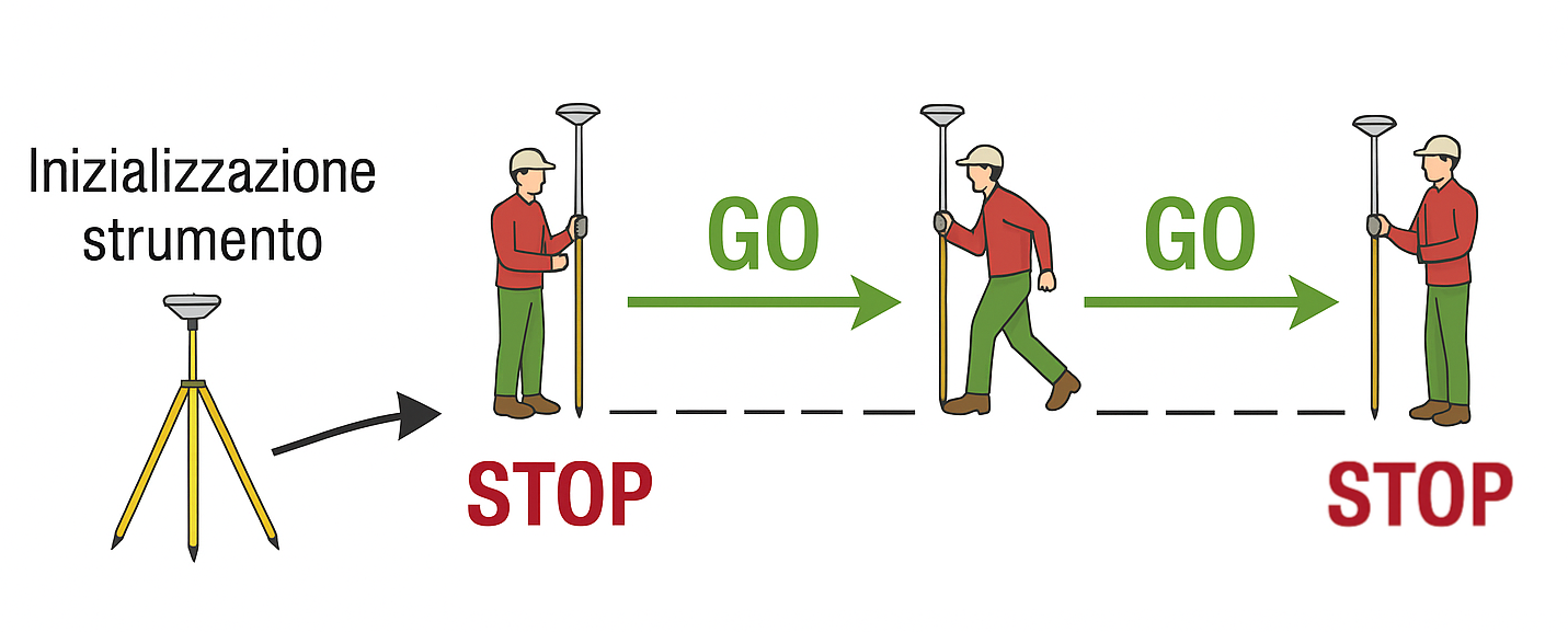
Fig.2 Surveying in kinematic Stop&Go mode
Advantages
- High accuracy (millimetre to centimetre).
- More flexible than pure static mode.
- Faster than a classic static survey.
Disadvantages
- Requires continuous visibility of the satellites and of the signal from the base.
- Requires an initial fixing stage and care not to lose the phase lock.
Equipment
- GNSS base (fixed): set up on a known point, it records RINEX data or transmits RTK corrections.
- GNSS rover (moving): receives the satellite data and the corrections from the base.
- Pole with bubble: to keep the point vertical.
- Bipod: to keep the pole vertical
- Controller with field software: to record points and metadata.
Applications
- Cadastral and high-precision surveys.
- Structural or environmental monitoring.
- Geodetic framing networks.
- Areas with no radio coverage (mountains, islands, remote areas).
The procedure
The figure below shows the main screen as it appears when you reach the web app through the link mentioned above
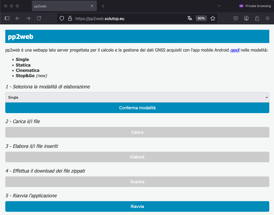
Fig.1 The web app at start-up
You then choose the raw data processing mode among single, static, kinematic and stop&go, as in the screen below
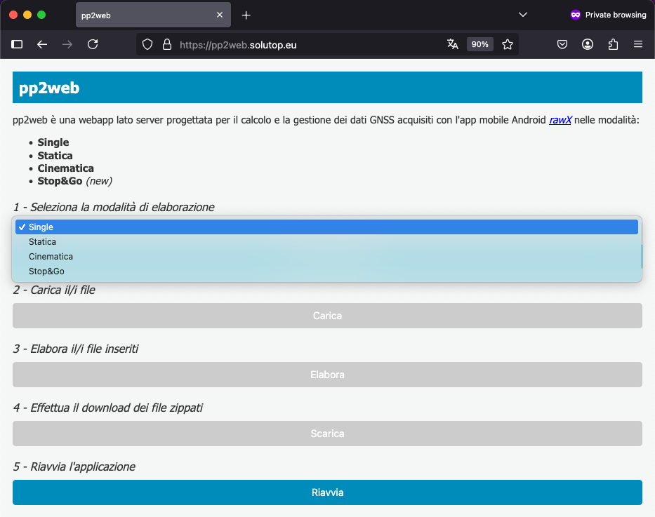
Fig.2 Choosing the processing mode
Confirm the mode and enter:
- the rover file in .ubx format
- the master file in .YYo or .obs format
- the file holding the stop and go intervals (stop&go mode only)
- the instrument height in metres, where applicable (single, static and kinematic modes only)
- the coordinates of the master, should you have them, as in fig. 3
Please note: the process is sequential, so the procedure cannot be carried out in the wrong order, as in fig. 3
Note
Note that single mode post-processes the rover .ubx file alone, since no master file is needed for that choice: the computation is a single-point solution (metre-level). It can be useful, for instance, to find the approximate coordinates of the recorded point in the WGS84 geographic system (L, L, E)
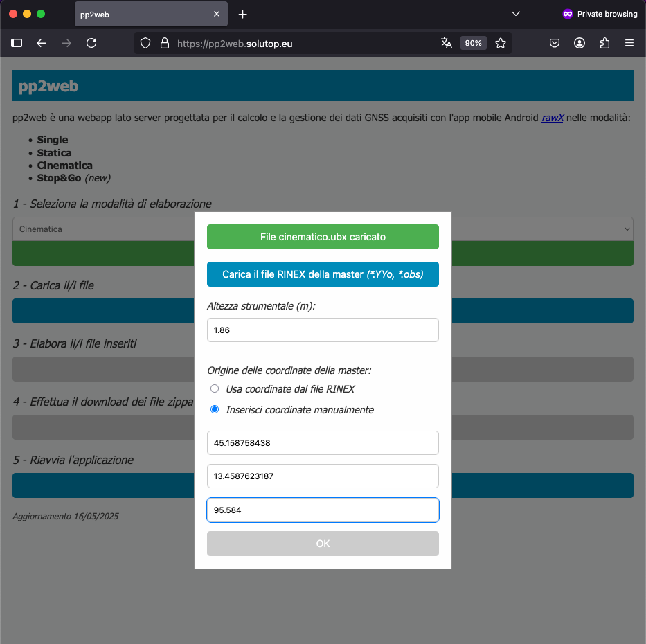
Fig.3 Importing the files and choosing the geographic coordinates
Note
If you have virtual RINEX files for static or kinematic post-processing, you will not have to enter LLE by hand to get the correct master coordinates: they are already precise, not approximate, in the header of the master RINEX file.
Below is an example of a RINEX file downloaded from a permanent master reference station; note the “APPROX POSITION XYZ” line of the header, highlighted below:
     2.11           OBSERVATION DATA    M (MIXED)           RINEX VERSION / TYPE
teqc  2016Apr1      OGS/CRS             20160608 12:19:48UTCPGM / RUN BY / DATE
Linux 2.4.21-27.ELsmp|Opteron|gcc|Linux x86_64|=+           COMMENT
BIT 2 OF LLI FLAGS DATA COLLECTED UNDER A/S CONDITION       COMMENT
UDI1                                                        MARKER NAME
12719M002                                                   MARKER NUMBER
David Zuliani       OGS/CRS                                 OBSERVER / AGENCY
618-01139           TPS NET-G3A         4.1 May,31,2013     REC # / TYPE / VERS
24204               ASH701945E_M    SCIT                    ANT # / TYPE
  4317305.9964  1016832.9984  4568261.5793                  APPROX POSITION XYZ
        0.0083        0.0000        0.0000                  ANTENNA: DELTA H/E/N
     1     1                                                WAVELENGTH FACT L1/2
     5    L1    L2    C1    P2    P1                        # / TYPES OF OBSERV
     1.0000                                                 INTERVAL
Forced Modulo Decimation to 1 seconds                       COMMENT
 SNR is mapped to RINEX snr flag value [0-9]                COMMENT
  L1 & L2: min(max(int(snr_dBHz/6), 0), 9)                  COMMENT
pseudorange smoothing corrections not applied               COMMENT
  2016     6     8    11     0    0.0000000     GPS         TIME OF FIRST OBS
    17                                                      LEAP SECONDS
                                                            END OF HEADER
Please note: the coordinates given are geocentric.
Once the files and any geographic coordinates of the master have been entered, the processing is started simply by clicking the “Process” button. The computation uses standard parameters and, for the time being, this version does not allow them to be edited. Any error messages are shown on screen and the processing button turns red, blocking the following stages, as in figure 4
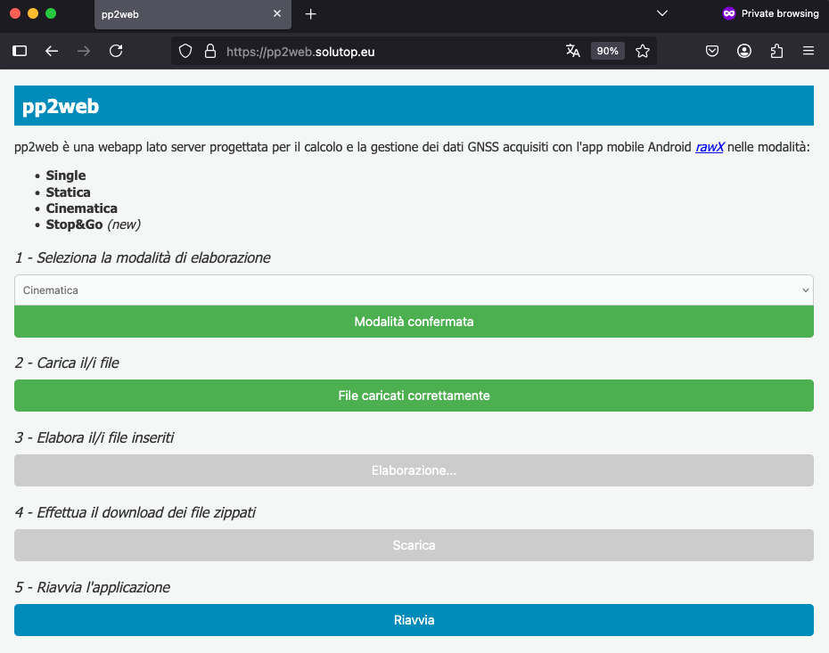
Fig.4 The uploaded files being processed
Once the processing is finished, the next step is the display of the points on an OSM map, which offers a first quick visual check of the data just processed. This stage is automatic and follows on from the previous one
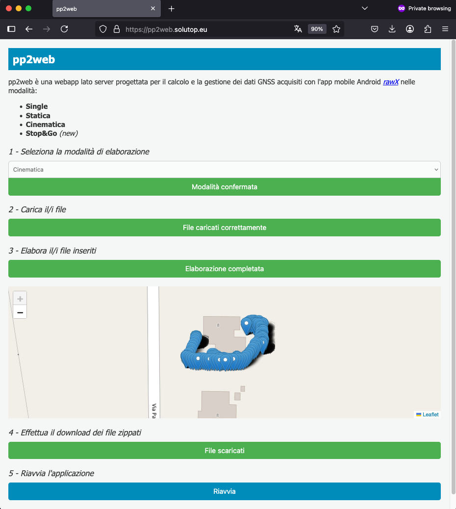
Fig.5 The result of the processing on the map
When this stage is over as well, the results can be downloaded as a zipped file holding:
- a .csv file with the coordinates of the fix solution alone for every epoch in single and static mode, plus the single coordinate for static mode, obtained as the weighted mean of all the coordinates with a fix solution
- a .pdf file with a detailed report, described in the next section
Final report
The final report describes the results of the processing as a whole and holds:
Observations and metadata (Observation Metadata)
- Overall duration of the observations
- Period expressed in UTC
- Mode
- Frequencies used
- Parameters: elevation mask, ionospheric corrections, tropospheric corrections, ephemerides
- Percentage of the solutions
- Satellites used
- Instrument height (single, static and kinematic modes only)
Kinematic track (GRD Track)
Position time series (Position Time Series)
Data summary (Data Summary)
Kinematic track
Figure 6 below shows an example of the plot representing the path followed by the GNSS receiver during the observation. It shows the movement of the device visually on a map (where available) or through a sequence of coordinates recorded in UTM, with the relevant zone chosen automatically.
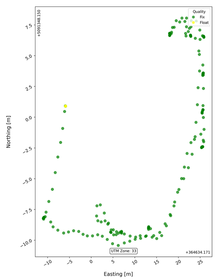
Fig.6 Plot of the planimetric E, N solution
Data provided:
- Geographic coordinates: latitude, longitude and elevation of the receiver
- Changes of position over time
- Quality of the solution (Fix/Float and so on)
- Possible graphical correlation with the map of the area
Purpose:
- Analysis of the trajectory and check of the path against its spatial context
Time series
Figure 7 below shows an example of the plot representing a detailed time series of the positions recorded by the GNSS receiver during the observation.
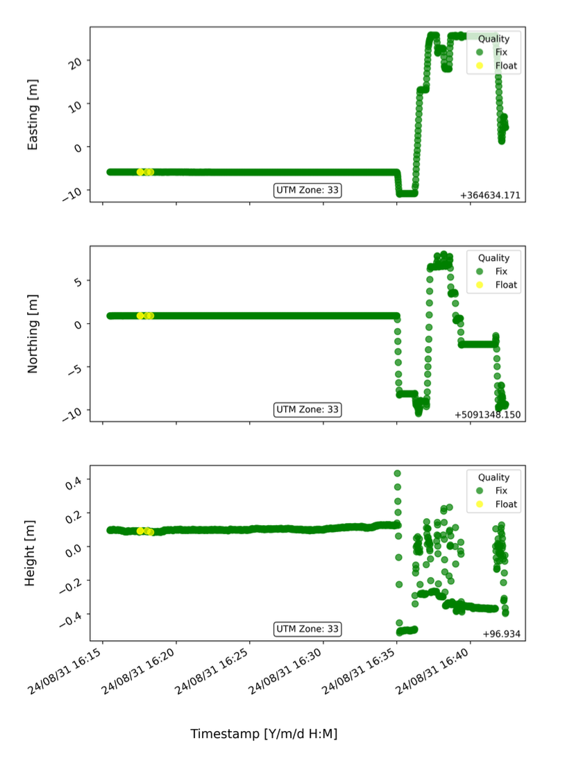
Fig.7 Plot of the E, N, H solution
Data provided:
- Timestamp: every position is tied to a specific time in UTC
- Coordinates: latitude, longitude and height (in metres)
- Precision: horizontal (SDH) and vertical (SDV) standard deviations
- Quality of the solution: every position is marked as Fix (high accuracy) or Float (lower accuracy)
Purpose:
- Detailed analysis of the quality of the measurements against time and the stability of the system.
Data summary
Figure 8 below shows part of an example of the overall summary of the observations and of the processing. Every single epoch is listed second by second, whatever the quality of the point.
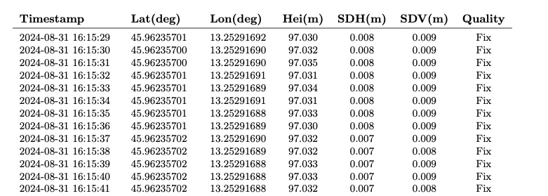
Fig.8 Summary of the post-processed epochs
Data provided:
- Overall statistics: total duration of the session with the individual positions epoch by epoch in LLE (deg)
- General precision: means and standard deviations of the horizontal and vertical measurements, and the solution epoch by epoch
Purpose:
- Concise assessment of the performance of the system and of the settings used
Note
The current version does not allow “parameter settings” — the choice of constellations, the ionospheric and tropospheric parameters, the cut-off angle and so on. For the sake of simplicity it uses a standard configuration file and converts the raw rover files at one-second intervals
In stop&go mode the Data Summary shows the instrument height as an extra column, as in fig. 9 below:
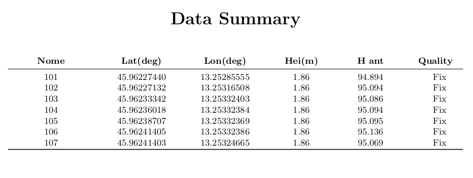
Fig.9 Summary with the points fixed in stop&go
Handling the timestamps
| Scale | Description | Example |
|---|---|---|
| UTC | Civil world time, includes leap seconds | 14:40:32 |
| GPST | Continuous GPS system time, starting on 6/1/1980, without leap seconds | 14:40:50 |
Current difference: GPST = UTC + 18 s (valid since 1/1/2017).
In its UBX messages the MS2 receiver always includes the leapS field, which carries the current 18 seconds, so that the software downstream can convert on its own.
┌─────────────────────────┐
│   Ricevitore  MS2       │
│  rcvTow + week + leapS  │
└────────────┬────────────┘
             │  stream binario UBX
             ▼
┌─────────────────────────┐                ┌──────────────────────┐
│   App Android  rawX     │   eventi       │   CSV Stop&Go        │
│                         ├───────────────►│   Timestamp UTC      │
│                         │                │   (orologio telefono)│
└────────────┬────────────┘                └──────────┬───────────┘
             │ raw bytes                              │
             ▼                                        │
┌─────────────────────────┐                           │
│   File  .ubx  (GPST)    │                           │
└────────────┬────────────┘                           │
             │                                        │
╔════════════▼════════════════════════╗               │
║  pp2web — post-processing           ║               │
║  (motore RTKLIB)                    ║               │
║                                     ║               │
║   UBX → RINEX (GPST)                ║               │
║   ↓                                 ║               │
║   PPK con out-timesys = utc         ║               │
║   ↓                                 ║               │
║   File .pos  (UTC) ◄── conversione  ║               │
║                       GPST→UTC      ║               │
║   ↓                                 ║               │
║   modulo Stop&Go                    ║◄──────────────┘
║   confronta CSV (UTC) con .pos (UTC)║
║   sulle finestre Stop→Go            ║
╚════════════════════╤════════════════╝
                     │
                     ▼
┌──────────────────────────────────────────┐
│  *_events_filtrato.csv                    │
│  *_events_media.csv  ← coordinate finali  │
└──────────────────────────────────────────┘
Data taken from a real field session on 19/06/2025.
# Modalità: Stop&Go
Point,Timestamp,Action,Height
1A,2025/06/19 14:40:32.925,Stop,2.07
1A,2025/06/19 14:41:32.945,Go,2.07
2A,2025/06/19 14:43:12.162,Stop,2.07
2A,2025/06/19 14:43:14.008,Go,2.07
The time is written in UTC from the phone’s clock.
| Field | Value |
|---|---|
rcvTow |
398,450.981 s (since the beginning of the GPS week) |
week |
2371 |
leapS |
18 |
| Reconstructed GPST | 2025-06-19T14:40:50.981 |
| UTC after subtracting leapS | 2025-06-19T14:40:32.981 |
| UTC | GPST | |
|---|---|---|
| Timestamp from the CSV | 14:40:32.925 |
— |
| Timestamp reconstructed from the UBX | 14:40:32.981 |
14:40:50.981 |
| Delta in UTC | +56 ms | |
| Delta in GPST | −18,056 ms |
The −18 seconds are exactly the leap seconds; the −56 ms are the small drift of the Android clock with respect to GPS time.
pp2web orchestrates three internal stages, using RTKLIB as its computation engine:
The .ubx file is turned into RINEX observations. At this stage the time is still GPS time: the observation file has not been converted to UTC.
This is where the key conversion happens. The internal configuration of pp2web tells RTKLIB out-timesys = utc: the engine reads the leap second supplied by the receiver and produces the .pos file with the epochs already in UTC. From this moment on, time is uniform: the same scale used by the event CSV.
pp2web takes the Stop → Go windows from the CSV and, for each of them, picks from the .pos file every epoch whose timestamp falls inside the interval. Over those epochs it computes the weighted mean of the coordinates (lat, lon, height), weighted by the inverse square of the standard deviations, and finally subtracts the instrument height of the point. Both streams (the CSV and the .pos epochs) are already in UTC, so no leap second correction is applied.
The “trick” is that every component of the pipeline does its job only once:
- rawX knows nothing about GPS: it writes civil UTC time.
- The MS2 receiver writes GPS time and attaches the leap second.
- pp2web (through RTKLIB) is the only component that converts between the two scales, and it does so once only, when the
.posfile is produced. - The stage that merges the Stop&Go events works in UTC alone, on two streams that are already consistent.
In other words: the responsibility for the GPST↔UTC conversion is centralised in pp2web, and rests on a single configuration line (out-timesys = utc) set internally.
| Symptom | Likely cause | Where to look |
|---|---|---|
The points in the .pos do not fall inside the CSV windows (off by about 18 s) |
pp2web configured with the wrong time system | the configuration file of the PPK processing |
| Occupations discarded with the message “at least 2-3 seconds” | rawX countdown too short | the countdown setting in the app |
| CSV-UBX delta greater than 1 second in UTC | Android clock out of sync | phone settings → automatic date and time |
| All solutions Q5 (single point) | the base RINEX does not cover the session | the time coverage of the base station |
- The 18 leap seconds must not be applied by hand: pp2web handles them through its internal configuration (
out-timesys = utcpassed to RTKLIB). - The rawX
.csvfile is natively in UTC (Android clock, NTP). - The
.posfile produced by pp2web is in UTC after the internal conversion. - The final merge of the Stop&Go events compares UTC with UTC: there is no risk of misalignment.
- The only thing left is the drift of the phone’s clock, typically a few tens of milliseconds — irrelevant for Stop&Go with occupations of 2 s or more.